27th July 2024

This submit takes up from two earlier posts (half 1;  half 2), asking simply what can we (we economists) actually find out about how rates of interest have an effect on inflation. At the moment, what does modern financial concept say? 

As you might recall, the usual story says that the Fed raises rates of interest; inflation (and anticipated inflation) do not instantly bounce up, so actual rates of interest rise; with some lag, increased actual rates of interest push down employment and output (IS); with some extra lag, the softer economic system results in decrease costs and wages (Phillips curve). So increased rates of interest decrease future inflation, albeit with “lengthy and variable lags.” 

Increased rates of interest -> (lag) decrease output, employment -> (lag) decrease inflation. 

Partly 1, we noticed that it isn’t simple to see that story within the information. Partly 2, we noticed that half a century of formal empirical work additionally leaves that conclusion on very shaky floor. 

As they are saying on the College of Chicago, “Effectively, a lot for the true world, how does it work in concept?” That is a crucial query. We by no means actually consider issues we do not have a concept for, and for good cause. So, at this time, let us take a look at what trendy concept has to say about this query. And they aren’t unrelated questions. Principle has been attempting to copy this story for many years. 

The reply: Fashionable (something submit 1972) concept actually doesn’t assist this concept. The usual new-Keynesian mannequin doesn’t produce something like the usual story.  Fashions that modify that easy mannequin to realize one thing like results of the usual story achieve this with an extended checklist of complicated components. The brand new components will not be simply adequate, they’re (apparently) obligatory to supply the specified dynamic sample. Even these fashions don’t  implement the verbal logic above. If the sample that prime rates of interest decrease inflation over just a few years is true, it’s by a very completely different mechanism than the story tells. 

I conclude that we do not have a easy financial mannequin that produces the usual perception. (“Easy” and “financial” are vital qualifiers.) 

The easy new-Keynesian mannequin 

The central downside comes from the Phillips curve. The fashionable Phillips curve asserts that price-setters are forward-looking. In the event that they know inflation will probably be excessive subsequent yr, they increase costs now. So 

Inflation at this time = anticipated inflation subsequent yr + (coefficient) x output hole.  

[pi_t = E_tpi_{t+1} + kappa x_t](If sufficient to complain about (betaapprox0.99) in entrance of (E_tpi_{t+1}) sufficient that it does not matter for the problems right here.)

Now, if the Fed raises rates of interest, and if (if) that lowers output or raises unemployment, inflation at this time goes down. 

The difficulty is, that is not what we’re searching for. Inflation goes down at this time, ((pi_t))relative to anticipated inflation subsequent yr ((E_tpi_{t+1})). So a better rate of interest and decrease output correlate with inflation that’s rising over time.    

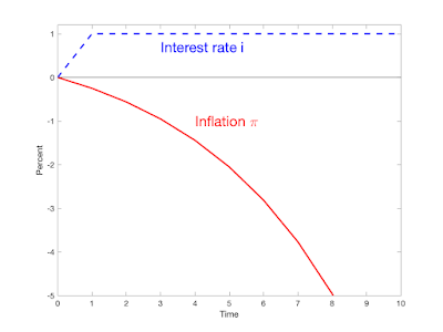
Here’s a concrete instance: 

The plot is the response of the usual three equation new-Keynesian mannequin to an (varepsilon_1) shock at time 1:[begin{align} x_t &= E_t x_{t+1} – sigma(i_t – E_tpi_{t+1}) pi_t & = beta E_t pi_{t+1} + kappa x_t i_t &= phi pi_t + u_t u_t &= eta u_{t-1} + varepsilon_t. end{align}] Right here (x) is output, (i) is the rate of interest, (pi) is inflation, (eta=0.6), (sigma=1), (kappa=0.25), (beta=0.95), (phi=1.2). 

On this plot, increased rates of interest are mentioned to decrease inflation. However they decrease inflation instantly, on the day of the rate of interest shock. Then, as defined above, inflation rises over time. 

In the usual view, and the empirical estimates from the final submit, a better rate of interest has no rapid impact, after which future inflation is decrease. See plots within the final submit, or this one from Romer and Romer’s 2023 abstract:

Inflation leaping down after which rising sooner or later is sort of completely different from inflation that does nothing instantly, would possibly even rise for just a few months, after which begins gently taking place. 

You would possibly even surprise concerning the downward bounce in inflation. The Phillips curve makes it clear why present inflation is decrease than anticipated future inflation, however why does not present inflation keep the identical, and even rise, and anticipated future inflation rise extra? That is the “equilibrium choice” challenge. All these paths are potential, and also you want further guidelines to choose a selected one. Fiscal concept factors out that the downward bounce wants a fiscal tightening, so represents a joint monetary-fiscal coverage. However we do not argue about that at this time. Take the usual new Keynesian mannequin precisely as is, with passive fiscal coverage and customary equilibrium choice guidelines. It predicts that inflation jumps down instantly after which rises over time. It doesn’t predict that inflation slowly declines over time.  

This isn’t a brand new challenge. Larry Ball (1994) first  identified that the usual new Keynesian Phillips curve says that inflation is excessive when inflation is excessive relative to anticipated future inflation, that’s when inflation is declining. Normal beliefs  go the opposite method: output is excessive when inflation is rising.  

The IS curve is a key a part of the general prediction, and output faces an analogous downside. I simply assumed above that output falls when rates of interest rise. Within the mannequin it does; output follows a path with the identical form as inflation in my little plot. Output additionally jumps down after which rises over time. Right here too, the (a lot stronger) empirical proof says that an rate of interest rise doesn’t change output instantly, and output then falls moderately than rises over time. The instinct has even clearer economics behind it: Increased actual rates of interest induce folks to eat much less at this time and extra tomorrow. Increased actual rates of interest ought to go together with increased, not decrease, future consumption development. Once more, the mannequin solely apparently reverses the signal by having output bounce down earlier than rising. 

Key points

How can we be right here, 40 years later, and the benchmark textbook mannequin so totally doesn’t replicate customary beliefs about financial coverage? 

One reply, I consider, is complicated adjustment to equilibrium with equilibrium dynamics. The mannequin generates inflation decrease than yesterday (time Zero to time 1) and decrease than it in any other case can be (time 1 with out shock vs time 1 with shock). Now, all financial fashions are a bit stylized. It is simple to say that once we add varied frictions, “decrease than yesterday” or “decrease than it will have been” is an efficient parable for “goes down over time.”  If in a easy provide and demand graph we are saying that a rise in demand raises costs immediately, we naturally perceive that as a parable for a drawn out interval of value will increase as soon as we add acceptable frictions. 

However dynamic macroeconomics does not work that method. We now have already added what was imagined to be the central friction, sticky costs. Dynamic economics is meant to explain the time-path of variables already, with no further parables. If adjustment to equilibrium takes time, then mannequin that.  

The IS and Phillips curve are ahead wanting, like inventory costs. It might make little sense to say “information comes out that the corporate won’t ever earn cash, so the inventory value ought to decline steadily over just a few years.” It ought to bounce down now. Inflation and output behave that method in the usual mannequin. 

A second confusion, I feel, is between sticky costs and sticky inflation. The brand new-Keynesian mannequin posits, and an enormous empirical literature examines, sticky costs. However that isn’t the identical factor as sticky inflation. Costs will be arbitrarily sticky and inflation, the primary by-product of costs, can nonetheless bounce. Within the Calvo mannequin, think about that solely a tiny fraction of corporations can change costs at every prompt. However after they do, they’ll change costs quite a bit, and the general value degree will begin growing immediately. Within the continuous-time model of the mannequin, costs are steady (sticky), however inflation jumps in the intervening time of the shock.  

The usual story needs sticky inflation. Many authors clarify the new-Keynesian mannequin with sentences like “the Fed raises rates of interest. Costs are sticky, so inflation cannot go up immediately and actual rates of interest are increased.” That is fallacious. Inflation can rise immediately. In the usual new-Keynesian mannequin it does so with (eta=1), for any quantity of value stickiness. Inflation rises instantly with a persistent financial coverage shock. 

Simply get it out of your heads. The usual mannequin doesn’t produce the usual story. 

The plain response is, let’s add components to the usual mannequin and see if we will modify the response perform to look one thing just like the widespread beliefs and VAR estimates. Let’s go. 

Adaptive expectations 

We will reproduce customary beliefs about financial coverage with completely adaptive expectations, within the 1970s ISLM kind. I feel it is a giant a part of what  most coverage makers and commenters keep in mind.  

Modify the above mannequin to go away out the dynamic a part of the intertemporal substitution equation, to simply say in moderately advert hoc method that increased actual rates of interest decrease output, and specify that the anticipated inflation that drives the true price and that drives pricing selections is mechanically equal to earlier inflation, (E_t pi_{t+1} = pi_{t-1}). We get [ begin{align} x_t &= -sigma (i_t – pi_{t-1}) pi_t & = pi_{t-1} + kappa x_t .end{align}] We will resolve this sytsem analytically to [pi_t = (1+sigmakappa)pi_{t-1} + sigmakappa i_t.]

Here is what occurs if the Fed completely raises the rate of interest. Increased rates of interest ship future inflation down. ((kappa=0.25, sigma=1.)) Inflation ultimately spirals away, however central banks do not go away rates of interest alone ceaselessly. If we add a Taylor rule response (i_t = phi pi_t + u_t),  so the central financial institution reacts to the rising spiral, we get this response to a everlasting financial coverage disturbance (u_t): 

The upper rate of interest units off a deflation spiral. However the Fed rapidly follows inflation right down to stabilize the scenario. That is, I feel, the traditional story of the 1980s. 

When it comes to components, an apparently minor change of index from (E_t pi_{t+1}) to (pi_{t-1}) is the truth is an enormous change. It means straight that increased output comes with growing inflation, not lowering inflation, fixing Ball’s puzzle.  The change mainly adjustments the signal of output within the Phillips curve. 
Once more, it is not likely all within the Phillips curve. This mannequin with rational expectations within the IS equation and adaptive within the Phillips curve produces junk. To get the consequence you want adaptive expectations in all places. 
The adaptive expectations mannequin will get the specified consequence by altering the essential signal and stability properties of the mannequin. Underneath rational expectations the mannequin is steady; inflation goes away all by itself beneath an rate of interest peg. With adaptive expectations, the mannequin is unstable. Inflation or deflation spiral away beneath an rate of interest peg or on the zero sure. The Fed’s job is like balancing a brush the wrong way up. Should you transfer the underside (rates of interest) a technique, the broom zooms off the opposite method. With rational expectations, the mannequin is steady, like a pendulum.  This isn’t a small wrinkle designed to switch dynamics. That is main surgical procedure. It’s also a sturdy property: small adjustments in parameters don’t change the dominant eigenvalue of a mannequin from over one to lower than one.  
A extra refined approach to seize how Fed officers and pundits assume and discuss is likely to be referred to as “briefly mounted expectations.” Coverage folks do discuss concerning the trendy Phillips curve; they are saying inflation depends upon inflation expectations and employment. Expectations will not be mechanically adaptive. Expectations are a 3rd pressure, generally “anchored,” and amenable to manipulation by speeches and dot plots. Crucially, on this evaluation, anticipated inflation doesn’t transfer when the Fed adjustments rates of interest.  Expectations are then  very slowly adaptive, if inflation is persistent, or if there’s a extra basic lack of religion in “anchoring.” Within the above new-Keynesian mannequin graph, on the minute the Fed raises the rate of interest, anticipated inflation jumps as much as comply with the graph’s plot of the mannequin’s forecast of inflation. 
As a easy approach to seize these beliefs, suppose expectations are mounted or “anchored” at (pi^e). Then my easy mannequin is [begin{align}x_t & = -sigma(i_t – pi^e) pi_t & = pi^e + kappa x_tend{align}]so [pi_t = pi^e – sigma kappa (i_t – pi^e).] Inflation is anticipated inflation, and lowered by increased rates of interest (final – signal). However these charges want solely be increased than the mounted expectations; they don’t must be increased than previous charges as they do within the adaptive expectations mannequin. That is why the Fed thinks 3% rates of interest with 5% inflation remains to be “contractionary”–expected inflation stays at 2%, not the 5% of latest adaptive expertise.  Additionally by fixing expectations, I take away the instability of the adaptive expectations mannequin… as long as these expectations keep anchored. The Fed acknowledges that ultimately increased inflation strikes the expectations, and with a perception that’s adaptive, they worry that an inflation spiral can nonetheless escape.
Even this view doesn’t give us any lags, nonetheless. The Fed and commenters clearly consider that increased actual rates of interest at this time decrease output subsequent yr, not instantly; and so they consider that decrease output and employment at this time drive inflation down sooner or later, not instantly. They consider one thing like [begin{align}x_{t+1} &= – sigma(i_t – pi^e) pi_{t+1} &= pi^e + kappa x_t.end{align}] 
However now we’re on the type of non-economic ad-hockery that the entire 1970s revolution deserted. And for a cause: Advert hoc fashions are unstable, regimes are at all times altering. Furthermore, let me remind you of our quest: Is there a easy financial mannequin of financial coverage that generates one thing like the usual view? At this degree of ad-hockery you would possibly as nicely simply write down the coefficients of Romer and Romer’s response perform and name that the mannequin of how rates of interest have an effect on inflation.  
Educational economics gave up on mechanical expectations and ad-hoc fashions within the 1970s. You’ll be able to’t publish a paper with this kind of mannequin. So after I imply a “trendy” mannequin, I imply  rational expectations, or no less than the consistency situation that the expectations in the mannequin will not be basically completely different from forecasts of the mannequin. (Fashions with specific studying or different expectation-formation frictions depend too.) 
It is simple to puff about folks aren’t rational, and searching the window a number of folks do dumb issues. But when we take that view, then the entire challenge of financial coverage on the proposition that persons are basically unable to study patterns within the economic system, {that a} benevolent Federal Reserve can trick the poor little souls into a greater consequence.  And someway the Fed is the lone super-rational actor who can keep away from all these pesky behavioral biases. 
We’re searching for the minimal obligatory components to explain the essential indicators and performance of financial coverage. A little bit of irrational or complicated expectation formation as icing on the cake, a potential adequate ingredient to supply quantitatively sensible dynamics, is not terrible. However it will be unhappy if irrational expectations or different habits is a obligatory ingredient to get probably the most primary signal and story of financial coverage proper. If persistent irrationality is a central obligatory ingredient for the essential signal and operation of financial coverage — if increased rates of interest will increase inflation the minute folks smarten up; if there is no such thing as a easy provide and demand, MV=PY smart economics underlying the essential operation of financial coverage; if it is all a conjuring trick  — that ought to actually weaken our religion in the entire financial coverage challenge.  
Info assist, and we do not have to get non secular about it. In the course of the lengthy zero sure, the identical commentators and central bankers stored warning a few deflation spiral, clearly predicted by this mannequin. It by no means occurred. Rates of interest under inflation from 2021 to 2023 ought to have led to an upward inflation spiral. It by no means occurred — inflation eased all by itself with rates of interest under inflation.Getting the specified response to rates of interest by making the mannequin unstable is not tenable whether or not or not you just like the ingredient.  Inflation additionally surged within the 1970s quicker than adaptive expectations got here near predicting, and fell quicker within the 1980s.  The ends of many inflations include credible adjustments in regime. 
There may be loads of work now desperately attempting to repair new-Keynesian fashions by making them extra old-Keynesian, placing lagged inflation within the Phillips curve, present revenue within the IS equation, and so forth. Complicated studying and expectation formation tales substitute the simplistic adaptive expectations right here. So far as I can inform, to the extent they work they largely achieve this in the identical method, by reversing the essential stability of the mannequin. 
Modifying the new-Keynesian mannequin
The choice is so as to add components to the essential new-Keynesian mannequin, sustaining its insistence on actual “micro-founded” economics and forward-looking habits, and describing specific dynamics because the evolution of equilibrium portions.  
Christiano Eichenbaum and Evans (2005) is among the most well-known examples. Recall these similar authors  created the primary most influential VAR that gave the “proper” reply to the consequences of financial coverage shocks. This paper modifies the usual new-Keynesian mannequin with a particular eye to matching impulse response features. The wish to match all impulse-responses, with a particular give attention to output. Once I began asking my younger macro colleagues for the standard mannequin which produces the specified response form, they nonetheless cite CEE first, although it is 20 years later. That is fairly an accomplishment. I will have a look at it intimately, as the overall image is similar as many different fashions that obtain the specified consequence. 
The stable line is the VAR level estimate and grey shading is the 95% confidence band. The stable blue line is the primary mannequin. The dashed line is the mannequin with solely value stickiness, to emphasise the significance of wage stickiness. The shock occurs at time 0. Discover the funds price line that jumps down at that date. That the opposite traces don’t transfer at time Zero is a consequence. I graphed the response to a time 1 shock above. 
That is the reply, now what is the query? What components did they add above the textbook mannequin to reverse the essential signal and bounce downside and to supply  these fairly footage? Here’s a partial checklist: 
  • Behavior formation. The utility perform is  (log(c_t – bc_{t-1})). 
  • A capital inventory with adjustment prices in funding.  Adjustment prices are proportional to funding development, ([1-S(i_t/i_{t-1})]i_t), moderately than the same old formulation wherein adjustment prices are proportional to the funding to capital ratio (S(i_t/k_t)i_t). 
  • Variable capital utilization. Capital companies (k_t) are associated to the capital inventory (bar{ok}t) by (k_t = u_t bar{ok}_t). The utilization price (u_t) is ready by households going through an upward sloping value (a(u_t)bar{ok}_t).
  • Calvo pricing with indexation: Corporations randomly get to reset costs, however corporations that are not allowed to reset costs do routinely increase costs on the price of inflation.
  • Costs are additionally mounted for 1 / 4. Technically, corporations should submit costs earlier than they see the interval’s shocks.
  • Sticky wages, additionally with indexation. Households are monopoly suppliers of labor, and set wages Calvo-style like corporations. (Later papers put all households right into a union which does the wage setting.) Wages are additionally listed; Households that do not get to reoptimize their wage nonetheless increase wages following inflation. 
  • Corporations should borrow working capital to finance their wage invoice 1 / 4 prematurely, and thus pay a curiosity on the wage invoice. 
  • Cash within the utility perform, and cash provide management. Financial coverage is a change within the cash development price, not a pure rate of interest goal. 
Whew! However which of those components are obligatory, and that are simply adequate? Figuring out the authors, I  strongly suspect that they’re all essential to get the suite of outcomes. They do not add components for present. However they wish to match all the impulse response features, not simply the inflation response. Maybe an easier set of components might generate the inflation response whereas lacking among the others. 
Let’s perceive what every of those components is doing, which is able to assist us to see (if) they’re obligatory and important to getting the specified consequence. 
I see a standard theme in behavior formation, adjustment prices that scale by funding development, and indexation. These components every add a by-product; they take a normal relationship between ranges of financial variables and alter it to at least one in development charges. Every of consumption, funding, and inflation is a “bounce variable” in customary economics, like inventory costs. Consumption (roughly) jumps to the current worth of future revenue. The extent of funding is proportional to the inventory value in the usual q concept, and jumps when there’s new info. Iterating ahead the new-Keynesian Phillips curve (pi_t = beta E_t pi_{t+1} + kappa x_t), inflation jumps to the discounted sum of future output gaps, (pi_t = E_t sum_{j=0}^infty beta^jx_{t+j}.)  
To provide responses wherein output, consumption and funding in addition to inflation rise slowly after a shock, we do not need ranges of consumption, funding, and inflation to leap this manner. As a substitute we wish development charges to take action. With customary utility, the patron’s linearized first order situation equates anticipated consumption development to the rate of interest, ( E_t (c_{t+1}/c_t) = delta + r_t ) Behavior, with (b=1) offers  ( E_t [(c_{t+1}-c_t)/(c_t-c_{t-1})] = delta + r_t ). (I disregarded the strategic phrases.) Mixing logs and ranges a bit, you’ll be able to see we put a development price instead of a degree. (The paper has (b=0.65) .) An funding adjustment value perform with (S(i_t/i_{t-1})) moderately than the usual (S(i_t/k_t)) places a by-product instead of a degree. Usually we inform a narrative that if you need a home painted, doubling the variety of painters does not get the job executed twice as quick as a result of they get in one another’s method. However you’ll be able to double the variety of painters in a single day if you wish to achieve this. Right here the fee is on the enhance in variety of painters every day.   Indexation ends in a Phillips curve with a lagged inflation time period, and that provides “sticky inflation.”  The Phillips curve of the mannequin (32) and (33) is [pi_t = frac{1}{1+beta}pi_{t-1} + frac{beta}{1+beta}E_{t-1}pi_{t+1} + (text{constants}) E_{t-1}s_t]the place (s_t) are marginal prices (extra later). The (E_{t-1}) come from the idea that costs cannot react to time (t) info. Iterate that ahead to (33)[pi_t – pi_{t-1} = (text{constants}) E_{t-1}sum_{j=0}^infty beta^j s_{t+j}.] We now have efficiently put the change in inflation instead of the extent of inflation. 
The Phillips curve is anchored by actual marginal prices, and they aren’t proportional to output on this mannequin as they’re within the textbook mannequin above. That is vital too. As a substitute,[s_t = (text{constants}) (r^k_t)^alpha left(frac{W_t}{P_t}R_tright)^{1-alpha}] the place (r^ok) is the return to capital (W/P) is the true wage and (R) is the nominal rate of interest. The latter time period crops up from the idea that corporations should borrow the wage invoice one interval prematurely. 
That is an attention-grabbing ingredient. There may be loads of discuss that increased rates of interest increase prices for corporations, and they’re decreasing output consequently. Which may get us round among the IS curve issues. However that is not the way it works right here. 
Here is how I feel it really works. Increased rates of interest increase marginal prices, and thus push up present inflation relative to anticipated future inflation. The equilibrium-selection guidelines and the rule towards prompt value adjustments (developing subsequent) tie down present inflation, so the upper rates of interest must push down anticipated future inflation. 
CEE disagree (p. 28). Writing of an rate of interest decline, so all of the indicators are reverse of my tales,  
… the rate of interest seems in corporations’ marginal value. Because the rate of interest drops after an expansionary financial coverage shock, the mannequin embeds a pressure that pushes marginal prices down for a time frame. Certainly, within the estimated benchmark mannequin the impact is powerful sufficient to induce a transient fall in inflation.
However pushing marginal prices down lowers present inflation relative to future inflation — they’re wanting on the similar Phillips curve simply above. It appears to me like they’re complicated present with anticipated future inflation. Instinct is tough. There are many Fisherian forces on this mannequin that need decrease rates of interest to decrease inflation. 
Extra deeply,  we see right here a foundational bother of the Phillips curve. It was initially a statistical relation between wage inflation and unemployment. It turned a (weaker) statistical relation between value inflation and unemployment or the output hole. The brand new-Keynesian concept needs naturally to explain a relation between marginal prices and value adjustments, and it takes contortions to make output equal to marginal prices. Phillips curves match the information terribly. So authors estimating Phillips curves (An early favourite by Tim Cogley and Argia Sbordone) return, and separate marginal value from output or employment. As CEE write later, they “construct options into the mannequin which be certain that corporations’ marginal prices are almost acyclical.” That helps the match, but it surely divorces the Phillips curve shifter variable from the enterprise cycle! Normal doctrine says that for the Fed to decrease inflation it should soften the economic system and threat unemployment. Doves say do not do it, reside with inflation to keep away from that value. Effectively, if the Phillips curve shifter is “acyclical” you must throw all that out the window.  
This shift additionally factors to the central conundrum of the Phillips curve. Right here it describes the adjustment of costs to wages or “prices” extra usually. It basically describes a relative value, not a value degree. OK, however the phenomenon we wish to clarify is the widespread element, how all costs and wage tie collectively or equivalently the decline within the worth of the forex, stripped of relative value actions. The central puzzle of macroeconomics is why the widespread element, an increase or fall of all costs and wages collectively, has something to do with output, and for us how it’s managed by the Fed. 
Christiano Eichenbaum and Evans write (p.3) that “it’s essential to permit for variable capital utilization.” I will strive clarify  why in my very own phrases. With out capital adjustment prices, any change in the true return results in an enormous funding bounce. (r=f'(ok)) should bounce and that takes loads of further (ok). We add adjustment prices to tamp down the funding response. However now when there’s any shock, capital cannot regulate sufficient and there’s a huge price of return response. So we want one thing that acts like an enormous bounce within the capital inventory to tamp down (r=f'(ok)) variability, however not an enormous funding bounce. Variable capital utilization acts like the large funding bounce with out us seeing an enormous funding bounce. And all that is going to be vital for inflation too. Bear in mind the Phillips curve; if output jumps then inflation jumps too. 
Sticky wages are essential, and certainly CEE report that they will dispense with sticky costs. One cause is that in any other case income are countercyclical. In a increase, costs go up quicker than wages so income go up. With sticky costs and versatile wages you get the alternative signal. It is attention-grabbing that the “textbook” mannequin has not moved this manner. Once more, we do not typically sufficient write textbooks. 
Fixing costs and wages in the course of the interval of the shock by assuming value setters cannot see the shock for 1 / 4 has a direct impact: It stops any value or wage jumps in the course of the quarter of the shock, as in my first graph. That is virtually dishonest. Notice the VAR additionally has completely zero instantaneous inflation response. This too is by assumption. They “orthogonalize” the variables so that every one the contemporaneous correlation between financial coverage shocks and inflation or output is taken into account a part of the Fed’s “rule” and none of it displays within-quarter response of costs or portions to the Fed’s actions. 
Step again and admire. Given the challenge “discover embellishments of the usual new-Keynesian mannequin to match VAR impulse response features” might you may have provide you with any of this? 
However again to our job. That is loads of apparently obligatory components. And studying right here or CEE’s verbal instinct, the logic of this mannequin is nothing like the usual easy instinct, which incorporates not one of the obligatory components. Do we actually want all of this to supply the essential sample of financial coverage? So far as we all know, we do. 
And therefore, that sample will not be as strong because it appears. For all of those components are fairly, … imaginative. Actually, we’re a good distance from the Lucas/Prescott imaginative and prescient that macroeconomic fashions must be primarily based on nicely tried and measured microeconomic components which might be believably invariant to adjustments within the coverage regime. 
CEE argue arduous for the plausibility of those microeconomic specs (see particularly the later Journal of Financial Views article), however they must strive so arduous exactly as a result of the usual literature does not have any of those components. The “degree” moderately than “development price” foundations of consumption, funding, and pricing selections pervade microeconomics. 
Microeconomists fear about labor monopsony, not labor monopoly; corporations set wages not households. (Christiano Eichenbam and Trabandt (2016) get wage stickiness from a extra sensible search and matching mannequin. Curiously, the one huge labor union fiction remains to be the most typical, although few non-public sector staff are unionized.) Corporations do not borrow the wage invoice 1 / 4 forward of time.  Only a few costs and wages are listed within the US. Like habits, maybe these components are easy stand ins for one thing else, however sooner or later we have to know what that one thing else is. That’s very true if one needs to do optimum coverage or welfare evaluation. 
Simply how a lot economics should we reinvent to match this one response perform? How far are we actually from the ad-hoc ISLM equations that Sims (1980) destroyed? 
Sadly, subsequent literature does not assist a lot (extra under). Subsequent literature has largely added components, together with heterogeneous brokers (huge lately), borrowing constraints, further monetary frictions (particularly after 2008), zero sure constraints, QE, studying and complicated expectations dynamics. (See CEE 2018 JEP  for a superb verbal survey.) The rewards in our career go to those that add a brand new ingredient. It’s totally arduous to publish papers that strip a mannequin right down to its fundamentals. Editors do not depend that as “new analysis,” however simply “exposition” under the status of their journals. Although boiling a mannequin right down to necessities is possibly extra vital in the long run than including extra bells and whistles. 

That is about the place we’re. Regardless of the beautiful response features, I nonetheless rating that we do not have a dependable, easy, financial mannequin that produces the usual view of financial coverage. 

Mankiw and Reis, sticky expectations 

Mankiw and Reis (2002) expressed the problem clearly over 20 years in the past. In reference to the “customary” New-Keynesian Phillips curve (pi_t = beta E_t pi_{t+1} + kappa x_t) they write a ravishing and succinct paragraph: 

Ball [1994a] reveals that the mannequin yields the shocking consequence that introduced, credible disinflations trigger booms moderately than recessions. Fuhrer and Moore [1995] argue that it can’t clarify why inflation is so persistent. Mankiw [2001] notes that it has bother explaining why shocks to financial coverage have a delayed and gradual impact on inflation. These issues seem to come up from the identical supply: though the value degree is sticky on this mannequin, the inflation price can change rapidly. In contrast, empirical analyses of the inflation course of (e.g., Gordon [1997]) sometimes give a big position to “inflation inertia.”

At the price of repetition, I emphasize the final sentence as a result of it’s so ignored. Sticky costs will not be sticky inflation. Ball already mentioned this in 1994: 

Taylor (1979, 198) and Blanchard (1983, 1986) present that staggering produces inertia within the value degree: costs simply slowly to a fall in th cash provide. …Disinflation, nonetheless, is a change within the development price of cash not a one-time shock to the extent. In casual discussions, analysts typically assume that the inertia consequence carries over from ranges to development charges — that inflation adjusts slowly to a fall in cash development. 

As I see it, Mankiw and Reis generalize the Lucas (1972) Phillips curve. For Lucas, roughly, output is expounded to sudden inflation[pi_t = E_{t-1}pi_t + kappa x_t.] Corporations do not see everybody else’s costs within the interval. Thus, when a agency sees an sudden rise in costs, it does not know if it’s a increased relative value or a better basic value degree; the agency expands output primarily based on how a lot it thinks the occasion is likely to be a relative value enhance.  I really like this mannequin for a lot of causes, however one, which appears to have fallen by the wayside, is that it explicitly founds the Phillips curve in corporations’ confusion about relative  costs vs. the value degree, and thus faces as much as the issue why ought to an increase within the value degree have any actual results. 

Mankiw and Reis mainly suppose that corporations discover out the overall value degree with lags, so output depends upon inflation relative to a distributed lag of its expectations. It is clearest for the value degree (p. 1300)[p_t = lambdasum_{j=0}^infty (1-lambda)^j E_{t-j}(p_t + alpha x_t).] The inflation expression is [pi_t = frac{alpha lambda}{1-lambda}x_t + lambda sum_{j=0}^infty (1-lambda)^j E_{t-1-j}(pi_t + alpha Delta x_t).](A few of the complication is that you really want it to be (pi_t = sum_{j=0}^infty E_{t-1-j}pi_t + kappa x_t), however output does not enter that method.) 

This appears completely pure and smart to me. What’s a “interval” anyway? It is sensible that corporations study heterogeneously whether or not a value enhance is relative or value degree. And it clearly solves the central persistence downside with the Lucas (1972) mannequin, that it solely produces a one-period output motion. Effectively, what’s a interval anyway? (Mankiw and Reis do not promote it this manner, and really do not cite Lucas in any respect. Curious.)  

It is not instantly apparent that this curve solves the Ball puzzle and the declining inflation puzzle, and certainly one should put it in a full mannequin to take action. Mankiw and Reis (2002) combine it with (m_t + v = p_t + x_t) and make some stylized evaluation, however do not present the way to put the thought in fashions comparable to I began with or make a plot.  

Their much less well-known comply with on paper  Sticky Info in Common Equilibrium (2007) is a lot better for this function as a result of they do present you the way to put the thought in an specific new-Keynesian mannequin, just like the one I began with.  Additionally they add a Taylor rule, and an rate of interest moderately than cash provide instrument, together with wage stickiness and some different components,. They present the way to resolve the mannequin overcoming the issue that there are lots of lagged expectations as state variables. However right here is the response to the financial coverage shock: 

Response to a Financial Coverage Shock, Mankiw and Reis (2007). 

Sadly they do not report how rates of interest reply to the shock. I presume rates of interest went down briefly. 

Look: the inflation and output hole plots are about the identical. Apart from the slight delay going up, these are precisely the responses of the usual NK mannequin. When output is excessive, inflation is excessive and declining.  The entire level was to supply a mannequin wherein excessive output degree would correspond to rising inflation. Relative to the primary graph, the primary enchancment is only a slight hump form in each inflation and output responses. 

Describing the identical mannequin in “Pervasive Stickiness” (2006), Mankiw and Reis describe the desideratum nicely: 

The Acceleration Phenomenon….inflation tends to rise when the economic system is booming and falls when financial exercise is depressed. That is the central perception of the empirical literature on the Phillips curve. One easy approach to illustrate this reality is to correlate the change in inflation, (pi_{t+2}-pi_{t-2}) with [the level of] output, (y_t), detrended with the HP filter. In U.S. quarterly information from 1954-Q3 to 2005-Q3, the correlation is 0.47. That’s, the change in inflation is procyclical.

Now look once more on the graph. So far as I  can see, it isn’t there. Is that this model of sticky inflation a bust, for this function? 

I nonetheless assume it is a neat concept price extra exploration. However I believed so 20 years in the past too.  Mankiw and Reis have loads of citations however no one adopted them. Why not?  I believe it is a part of a basic sample that a number of nice micro sticky value papers will not be used as a result of they do not produce a straightforward combination Phillips curve. In order for you cites, be sure that folks can plug it in to Dynare. Mankiw and Reis’ curve is fairly easy, however you continue to must maintain all previous expectations round as a state variable. There could also be other ways of doing that with trendy computational expertise, placing it in a Markov atmosphere or reducing off the lags, everybody learns the value degree after 5 years. Hank fashions have even larger state areas! 

Some extra fashions

What about throughout the Fed?  Chung,  Kiley, and  Laforte 2010, “Documentation of the Estimated, Dynamic, Optimization-based (EDO) Mannequin of the U.S. Financial system: 2010 Model” is one such mannequin.  (Because of Ben Moll, in a lecture slide titled “Results of rate of interest hike in U.S. Fed’s personal New Keynesian mannequin”) They describe it as 

This paper supplies documentation for a large-scale estimated DSGE mannequin of the U.S. economic system – the Federal Reserve Board’s Estimated, Dynamic, Optimization- primarily based (FRB/EDO) mannequin challenge. The mannequin can be utilized to deal with a variety of sensible coverage questions on a routine foundation.

Listed below are the central plots for our function: The response of rates of interest and inflation to a financial coverage shock.  

No lengthy and variable lags right here. Simply as within the easy mannequin, inflation jumps down on the day of the shock after which reverts. As with Mankiw and Reis, there’s a tiny hump form, however that is it. That is nothing just like the Romer and Romer plot. 

Smets and Wouters (2007) “Shocks and Frictions in US Enterprise Cycles: A Bayesian DSGE Method” is about as well-known as Christiano Eichenbaum and Evans as a normal new-Keynesian mannequin that supposedly matches information nicely. It “comprises many shocks and frictions. It options sticky nominal value and wage settings that permit for backward inflation indexation, behavior formation in consumption, and funding adjustment prices that create hump-shaped responses… and variable capital utilization and glued prices in manufacturing”
Right here is their central graph of the response to a financial coverage shock

Once more, there’s a little hump-shape, however the general image is rather like the one we began with. Inflation largely jumps down instantly after which recovers; the rate of interest shock results in future inflation that’s increased, not decrease than present inflation. There are not any lags from increased rates of interest to future inflation declines. 
Closing ideas

I will reiterate the primary level. So far as I can inform, there is no such thing as a easy financial mannequin that produces the usual perception. 

Now, possibly perception is true and fashions simply must catch up. It’s attention-grabbing that there’s so little effort happening to do that. As above, the huge outpouring of new-Keynesian modeling has been so as to add much more components. Partly, once more, that is the pure pressures of journal publication. However I feel it is also an sincere feeling that after Christiano Eichenbaun and Evans, it is a solved downside and including different components is all there’s to do. 

So a part of the purpose of this submit (and “Expectations and the neutrality of rates of interest”) is to argue that that is not a solved downside, and that eradicating components to search out the only financial mannequin that may produce customary beliefs is a very vital job.  Then, does the mannequin incorporate something at all the customary instinct, or is it primarily based on some completely different mechanism al collectively? These are first order vital and unresolved questions!

However for my lay readers, right here is so far as I do know the place we’re. Should you, just like the Fed, maintain to plain beliefs that increased rates of interest decrease future output and inflation with lengthy and variable lags, know there is no such thing as a easy financial concept behind that perception, and definitely the usual story isn’t how financial fashions of the final 4 a long time work. 

Leave a Reply

Your email address will not be published. Required fields are marked *

This site uses Akismet to reduce spam. Learn how your comment data is processed.