At the moment, I will add an entry to my occasional critiques of fascinating educational papers. The paper: “Worth Degree and Inflation Dynamics in Heterogeneous Agent Economies,” by Greg Kaplan, Georgios Nikolakoudis and Gianluca Violante.
One of many many causes I’m enthusiastic about this paper is that it unites fiscal principle of the value degree with heterogeneous agent economics. And it exhibits how heterogeneity issues. There was quite a lot of work on “heterogeneous agent new-Keynesian” fashions (HANK). This paper inaugurates heterogeneous agent fiscal principle fashions. Let’s name them HAFT.
The paper has a superbly stripped down mannequin. Costs are versatile, and the value degree is ready by fiscal principle. Folks face uninsurable revenue shocks, nonetheless, and a borrowing restrict. So that they save an additional quantity with a view to self-insure towards unhealthy occasions. Authorities bonds are the one asset within the mannequin, so this further saving pushes down the rate of interest, low cost charge, and authorities service debt value. The mannequin has a time-zero shock after which no mixture uncertainty.
That is precisely the appropriate place to start out. Ultimately, after all, we would like fiscal principle, heterogeneous brokers, and sticky costs so as to add inflation dynamics. And on prime of that, no matter DSGE smorgasbord is vital to the problems at hand; manufacturing facet, worldwide commerce, a number of actual belongings, monetary fractions, and extra. However the genius of an awesome paper is to start out with the minimal mannequin.
Half II results of fiscal shocks.
I’m most excited by half II, the consequences of fiscal shocks. This goes straight to vital coverage questions.
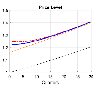 |
|
Be aware: This determine plots impulse responses to a focused and untargeted helicopter drop, aggregated on the quarterly frequency. The helicopter drop is a one-time issuance of 16% of whole authorities nominal debt excellent at t = 0. Solely households within the backside 60% of the wealth distribution obtain the issuance within the focused experiment (dashed crimson line). The orange line plots dynamics within the consultant agent (RA) mannequin. The dashed black line plots the preliminary regular state. Supply: Kaplan et al. Determine 7 |
At time 0, the federal government drops $5 trillion of additional debt on folks, with no plans to pay it again. The rate of interest doesn’t change. What occurs? Within the consultant agent financial system, the value degree jumps, simply sufficient to inflate away excellent debt by $5 trillion.
(On this simulation, inflation subsequent to the value degree bounce is simply set by the central financial institution, by way of an rate of interest goal. So the rising value degree line of the consultant agent (orange) benchmark will not be that fascinating. It isn’t a traditional impulse response displaying the change after the shock; it is the precise path after the shock. The distinction between coloured heterogeneous agent strains and the orange consultant agent line is the vital half.)
Punchline: Within the heterogeneous agent economies, the value degree jumps a superb deal extra. And if transfers are focused to the underside of the wealth distribution, the value degree jumps extra nonetheless. It issues who will get the cash.
This is step one on an vital coverage query. Why was the 2020-2021 stimulus a lot extra inflationary than, say 2008? I’ve quite a lot of tales (“fiscal histories,” FTPL), one among which is a imprecise sense that printing cash and sending folks checks has extra impact than borrowing in treasury markets and spending the outcomes. This graph makes that sense exact. Sending folks checks, particularly people who find themselves on the sting, does generate extra inflation.
Ultimately, whether or not authorities debt is inflationary or not comes down as to whether folks deal with the asset as a superb financial savings car, and hold on to it, or attempt to spend it, thereby driving up costs. Sending checks to folks prone to spend it offers extra inflation.
As you may see, the mannequin additionally introduces some dynamics, the place on this easy setup (versatile costs) the RA mannequin simply offers a value degree bounce. To grasp these dynamics, and extra instinct of the mannequin, take a look at the response of actual debt and the true rate of interest

The larger inflation implies that the identical improve in nominal debt is a lesser improve in actual debt. Now, the essential characteristic of the mannequin steps in: resulting from self-insurance, there’s primarily a liquidity worth of debt. You probably have much less debt, the marginal worth of upper; folks bid down the true rate of interest in an try and get extra debt. However the increased actual charge means the true worth of debt rises, and because the debt rises, the true rate of interest falls.
To grasp why that is the equilibrium, it is value wanting on the debt accumulation equation, [ frac{db}{dt} = r_t (b_t; g_t) b_t – s_t. ](b_t) is the true worth of nominal debt, (r_t=i_t-pi_t) is the true rate of interest, and (s_t) is the true main surplus. Greater actual charges (debt service prices) increase debt. Greater main surpluses pay down debt. Crucially — the entire level of the paper — the rate of interest is determined by how a lot debt is excellent and on the distribution of wealth (g_t). ((g_t) is a complete distribution.) Extra debt means the next rate of interest. Extra debt does a greater job of satisfying self-insurance motives. Then the marginal worth of debt is decrease, so folks do not attempt to save as a lot, and the rate of interest rises. It really works quite a bit like cash demand,
Now, if the switch had been proportional to present wealth, nothing would change, the value degree would bounce identical to the RA (orange) line. But it surely is not; in each instances more-constrained folks get more cash. The liquidity constraints are much less binding, they’re prepared to save lots of extra. For given mixture debt the true rate of interest will rise. So the orange line with no change in actual debt is now not a gentle state. We will need to have, initially (db/dt>0.) As soon as debt rises and the distribution of wealth mixes, we return to the outdated regular state, so actual debt rises much less initially, so it could possibly proceed to rise. And to try this, we want a bigger value degree bounce. Whew. (I hope I acquired that proper. Instinct is tough!)
In a earlier submit on heterogeneous agent fashions, I requested whether or not HA issues for aggregates, or whether or not it’s nearly distributional penalties of unchanged mixture dynamics. Right here is a superb instance during which HA issues for aggregates, each for the dimensions and for the dynamics of the consequences.
Here is a second cool simulation. What if, moderately than a lump-sum helicopter drop with no change in surpluses, the federal government simply begins working everlasting main deficits?
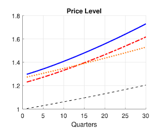 |
|
Be aware: Impulse response to a everlasting growth in main deficits. The dotted orange line exhibits the consequences of a discount in surplus within the Consultant Agent mannequin. The blue line labelled “Lump Sum” illustrates the dynamics following an growth of lump sum transfers. The dashed crimson line labelled “Tax Price” plots dynamics following a tax lower. The orange line plots dynamics within the consultant agent (RA) mannequin. The dashed black line plots the preliminary regular state. Supply: Kaplan et. al. Determine 8. |
Within the RA mannequin, a decline in surpluses is precisely the identical factor as an increase in debt. You get the preliminary value bounce, after which the identical inflation following the rate of interest goal. Not so the HA fashions! Perpetual deficits are totally different from a bounce in debt with no change in deficit.

Once more, actual debt and the true charge assist to know the instinct. The actual quantity of debt is completely decrease. Meaning persons are extra starved for buffer inventory belongings, and bid down the true rate of interest. The nominal charge is fastened, by assumption on this simulation, so a decrease actual charge means extra inflation.
For coverage, this is a crucial outcome. With versatile costs, RA fiscal principle solely offers a one-time value degree bounce in response to surprising fiscal shocks. It doesn’t give regular inflation in response to regular deficits. Right here we do have regular inflation in response to regular deficits! It additionally exhibits an occasion of the final “low cost charges matter” theorem. Granted, right here, the central financial institution may decrease inflation by simply reducing the nominal charge goal however we all know that is not really easy once we add realisms to the mannequin.
To see simply why that is the equilibrium, and why surpluses are totally different than debt, once more return to the debt accumulation equation, [ frac{db}{dt} = r_t (b_t, g_t) b_t – s_t. ] Within the RA mannequin, the value degree jumps in order that (b_t) jumps down, after which with smaller (s_t), (r b_t – s_t) is unchanged with a continuing (r). However within the HA mannequin, the decrease worth of (b) means much less liquidity worth of debt, and folks attempt to save, bidding down the rate of interest. We have to work down the debt demand curve, driving down the true curiosity prices (r) till they partially pay for among the deficits. There’s a sense during which “monetary repression” (artificially low rates of interest) by way of perpetual inflation assist to pay for perpetual deficits. Wow!
Half I r<g
The primary principle a part of the paper can also be fascinating. (Although these are actually two papers stapled collectively, since as I see it the idea within the first half is in no way obligatory for the simulations.) Right here, Kaplan, Nikolakoudis and Violante tackle the r<g query clearly. No, r<g doesn’t doom fiscal principle! I used to be so enthused by this that I wrote up just a little be aware “fiscal principle with detrimental rates of interest” right here. Detailed algebra of my factors beneath are in that be aware, (An essay r<g and in addition a r<g chapter in FTPL explains the associated situation, why it is a mistake to make use of averages from our actual financial system to calibrate excellent foresight fashions. Sure, we will observe (E(r)<E(g)) but current values converge.)
I will give the fundamental concept right here. To maintain it easy, take into consideration the query what occurs with a detrimental actual rate of interest (r<0), a continuing surplus (s) in an financial system with no progress, and ideal foresight. You would possibly assume we’re in hassle: [b_t = frac{B_t}{P_t} = int e^{-rtau} s dtau = frac{s}{r}.]A detrimental rate of interest makes current values blow up, no? Effectively, what a couple of completely detrimental surplus (s<0) financed by a completely detrimental curiosity value (r<0)? That sounds wonderful in circulation phrases, nevertheless it’s actually bizarre as a gift worth, no?
Sure, it’s bizarre. Debt accumulates at [frac{db_t}{dt} = r_t b_t – s_t.] If (r>0), (s>0), then the true worth of debt is generically explosive for any preliminary debt however (b_0=s/r). Due to the transversality situation ruling out actual explosions, the preliminary value degree jumps so (b_0=B_0/P_0=s/r). But when (r<0), (s<0), then debt is steady. For any (b_0), debt converges, the transversality situation is happy. We lose fiscal value degree dedication. No, you may’t take a gift worth of a detrimental cashflow stream with a detrimental low cost charge and get a wise current worth.
However (r) will not be fixed. The extra debt, the upper the rate of interest. So [frac{db_t}{dt} = r(b_t) b_t – s_t.] Linearizing across the regular state (b=s/r), [frac{db_t}{dt} = left[r_t + frac{dr(b_t)}{db}right]b_t – s.] So even when (r<0), if extra debt raises the rate of interest sufficient, if (dr(b)/db) is massive sufficient, dynamics are regionally and it seems globally unstable even with (r<0). Fiscal principle nonetheless works!
You possibly can work out a simple instance with bonds in utility, (int e^{-rho t}[u(c_t) + theta v(b_t)]dt), and simplifying additional log utility (u(c) + theta log(b)). On this case (r = rho – theta v'(b) = rho – theta/b) (see the be aware for derivation), so debt evolves as [frac{db}{dt} = left[rho – frac{theta}{b_t}right]b_t – s = rho b_t – theta – s.]Now the (r<0) half nonetheless offers steady dynamics and a number of equilibria. But when (theta>-s), then dynamics are once more explosive for all however (b=s/r) and monetary principle works anyway.
This can be a highly effective outcome. We often assume that in excellent foresight fashions, (r>g), (r>0) right here, and consequently constructive vs detrimental main surpluses (s>0) vs. (s<0) is a crucial dividing line. I do not know what number of fiscal principle critiques I’ve heard that say a) it does not work as a result of r<g so current values explode b) it does not work as a result of main surpluses are all the time barely detrimental.
That is all unsuitable. The evaluation, as on this instance, exhibits is that fiscal principle can work wonderful, and does not even discover, a transition from (r>0) to (r<0), from (s>0) to (s<0). Financing a gentle small detrimental main surplus with a gentle small detrimental rate of interest, or (r<g) is seamless.
The essential query on this instance is (s<-theta). At this boundary, there isn’t a equilibrium any extra. You possibly can finance solely a lot main deficit by monetary repression, i.e. squeezing down the quantity of debt so its liquidity worth is excessive, pushing down the curiosity prices of debt.
The paper staples these two workouts collectively, and calibrates the above simulations to (s<0) and (r<g). However I wager they’d look virtually precisely the identical with (s>0) and (r>g). (r<g) will not be important to the fiscal simulations.
The paper analyzes self-insurance towards idiosyncratic shocks as the reason for a liquidity worth of debt. That is fascinating, and permits the authors to calibrate the liquidity worth towards microeconomic observations on simply how a lot folks undergo such shocks and need to insure towards them. The Half I simulations are simply that, heterogeneous brokers in motion. However this theoretical level is way broader, and applies to any financial drive that pushes up the true rate of interest as the amount of debt rises. Bonds in utility, right here and within the paper’s appendix, work. They’re a standard stand in for the usefulness of presidency bonds in monetary transactions. And in that case, it is simpler to increase the evaluation to a capital inventory, actual property, overseas borrowing and lending, gold bars, crypto, and different technique of self-insuring towards shocks. Commonplace “crowding out” tales by which increased debt raises rates of interest work. (Blachard’s r<g work has quite a lot of such tales.) The “segmented markets” tales underlying religion in QE give a rising b(r). So the final precept is powerful to many various sorts of fashions.
My be aware explores one situation the paper doesn’t, and it is an vital one in asset pricing. OK, I see how dynamics are regionally unstable, however how do you’re taking a gift worth when r<0? If we write the regular state [b_t = int_{tau=0}^infty e^{-r tau}s dtau = int_{tau=0}^T e^{-r tau}s dtau + e^{-rT}b_{t+T}= (1-e^{-rT})frac{s}{r} + e^{-rT}b,]and with (r<0) and (s<0), the integral and ultimate time period of the current worth formulation every explode to infinity. It appears you actually cannot low cost with a detrimental charge.
The reply is: do not combine ahead [frac{db_t}{dt}=r b_t – s ]to the nonsense [ b_t = int e^{-r tau} s dtau.]As a substitute, combine ahead [frac{db_t}{dt} = rho b_t – theta – s]to [b_t = int e^{-rho tau} (s + theta)dt = int e^{-rho tau} frac{u'(c_t+tau)}{u'(c_t)}(s + theta)dt.]Within the final equation I put consumption ((c_t=1) within the mannequin) for readability.
- Low cost the circulation worth of liquidity advantages on the shopper’s intertemporal marginal charge of substitution. Don’t use liquidity to supply an altered low cost charge.
That is one other deep, and often violated level. Our low cost issue tips don’t work in infinite-horizon fashions. (1=E(R_{t+1}^{-1}R_{t+1})) works simply in addition to (1 = Eleft[beta u'(c_{t+1})/u'(c_t)right] r_{t+1}) in a finite horizon mannequin, however you may’t all the time use (m_{t+1}=R_{t+1}^{-1}) in infinite interval fashions. The integrals blow up, as within the instance.
This can be a good thesis subject for a theoretically minded researcher. It is one thing about Hilbert areas. Although I wrote the low cost issue e-book, I do not know the way to prolong low cost issue tips to infinite intervals. So far as I can inform, no person else does both. It isn’t in Duffie’s e-book.
Within the meantime, when you use low cost issue tips like affine fashions — something however the correct SDF — to low cost an infinite cashflow, and you discover “puzzles,” and “bubbles,” you are on skinny ice. There are many papers making this error.
A minor criticism: The paper does not present nuts and bolts of the way to calculate a HAFT mannequin, even within the easiest instance. Be aware against this how trivial it’s to calculate a bonds in utility mannequin that will get a lot of the similar outcomes. Give us a recipe e-book for calculating textbook examples, please!
Clearly it is a first step. As FTPL rapidly provides sticky costs to get cheap inflation dynamics, so ought to HAFT. For FTPL (or FTMP, fiscal principle of financial coverage; i.e. including rate of interest targets), including sticky costs made the story far more life like: We get a yr or two of regular inflation consuming away at bond values, moderately than a value degree bounce. I can not wait to see HAFT with sticky costs. For all the opposite requests for generalization: you simply discovered your thesis subject.
Ship typos, particularly in equations.